User Guide
This guide is an instruction manual on the RAPOC (Rosseland And Planck Opacity Converter) tool and how it can be included in one’s own code.
For a quickstart, please refer to the python notebook inside the examples directory. If RAPOC has been installed from Pypi, an example notebook can be found on the GitHub repository.
Input
Everything inside RAPOC is managed by the Model class.
The only input required by RAPOC is the opacity data.
Opacity data can be directly downloaded from dedicated repositories such as ExoMol or, instead,
by a custom made Python dictionary. In this guide both approaches will be explored:
Using ExoMol (easier)
This is the most straightforward approach.
Note that RAPOC only accepts data with the TauRex format.
Once the opacities have been downloaded from ExoMol,
RAPOC will load them using the ExoMolFileLoader.
For practice, we use the TauRex formatted opacities for water.
However, if other molecules are required then they can be downloaded here.
Using Dace
This is another straightforward approach.
The opacities can be downloaded from Dace as binary files.
RAPOC will load them using the DACEFileLoader by pointing to the directory
where the binary files (.bin) are stored.
Python dictionary (harder)
To load data from a Python dictionary, the code uses the DictLoader class.
The user may also refer to its documentation.
To summarise, the python dictionary must have the layout described in the Input data layout.
Input data layout¶ Information
data format
supported keys names
molecular name
string
mol
pressure grid in [\(Pa\)]
list or np.array
p, P, pressure, pressure_grid
temperature grid [\(K\)]
list or np.array
t, T, temperature, temperature_grid
wavenumber grid [\(1/cm\)]
list or np.array
wn, wavenumber, wavenumbers, wavenumbers_grid, wavenumber_grid
opacities [\(m^2/kg\)]
list or np.array
opacities
Every value in the dictionary can be assigned units by using the units astropy.units.Quantity.
The model
In this section we will assume that the data has been downloaded from ExoMol and that the input_file variable is a string pointing to that file.
Once the data is ready, it may loaded into the Model class.
After this, two classes can be produced, one for Rosseland and the other for Planck mean opacities:
Rosseland, Planck. These models can be initialised as such:
from rapoc import Rosseland, Planck

ross = Rosseland(input_data=input_file)
plan = Planck(input_data=input_file)
Normally, the molecule name is automatically extracted from the input data. However, if the molecule name is not present in the input data or if any errors occur, it can be manually set using the molecule keyword argument:
ross = Rosseland(input_data=input_file, molecule='H2O')
plan = Planck(input_data=input_file, molecule='H2O')
Calculating the mean opacities
For purely illustrative purposes, a temperature (T) of 1000 K with a pressure (P) of 1000 Pa in the wavelength range of 1-10 micron will be used. Therefore, the first step is to define the temperature, pressure and wavelength range:
import astropy.units as u

P = 1000.0 *u.Pa
T = 1000.0 *u.K
wl = (1 * u.um, 10 * u.um)
Due to the units provided by the astropy.units.Quantity module, RAPOC can handle the conversions automatically.
To perform the opacity calculations the following function is used: estimate()
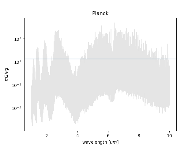
r_estimate = ross.estimate(P_input = P, T_input=T, band=wl, mode='closest')

0.00418 m2 / kg
p_estimate = plan.estimate(P_input = P, T_input=T, band=wl, mode='closest') 17.9466 m2 / kg
The investigated wavelength range may also be expressed as a wavenumbers range or frequencies range. This is achieved by attaching the corresponding units.
There are two estimation modes available in RAPOC:
closest: the code estimates the mean opacity for the closest pressure and temperature values found within the input data grid.
linear or loglinear: the code estimates the mean opacity by performing an interpolation that makes use of the
scipy.interpolate.griddata().
In the second case, RAPOC needs to first build a map() of the mean opacities
in the input pressure and temperature data grid.
This may be slow. To make this process faster, RAPOC will continue to reuse this map until the user
asks for estimates in another wavelength range. Only then would RAPOC produce a new map.
RAPOC can also perform estimates of multiple temperatures and pressures at once (e.g. lists and arrays):
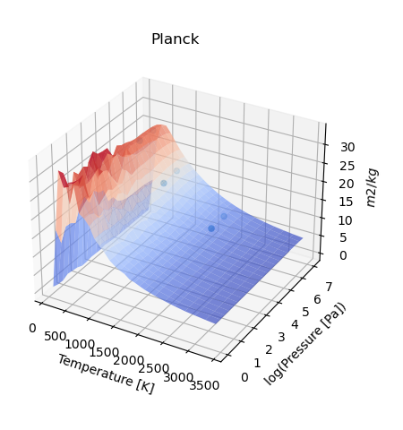
P = [1, 10 ] *u.bar
T = [500.0, 1000.0, 2000.0] *u.K
wl = (1 * u.um, 10 * u.um)

r_estimate = ross.estimate(P_input = P, T_input=T, band=wl, mode='closest')

[[0.00094728 0.03303942 0.17086334]
 [0.00484263 0.08600765 0.21673218]] m2 / kg
p_estimate = plan.estimate(P_input = P, T_input=T, band=wl, mode='closest') [[27.18478963 17.36108261 8.57782242] [27.17086583 17.78923892 8.8249388 ]] m2 / kg
Build some plots
RAPOC can build plots of the calculated Rosseland and Planck mean opacities by using estimate_plot().
If only a single value has been produced, then to produce plots one can use the following script:
P = 1000.0 *u.Pa
T = 1000.0 *u.K
wl = (1 * u.um, 10 * u.um)

fig0, ax0 = ross.estimate_plot(P_input = P, T_input=T, band=wl, mode='closest')
fig1, ax1 = plan.estimate_plot(P_input = P, T_input=T, band=wl, mode='closest')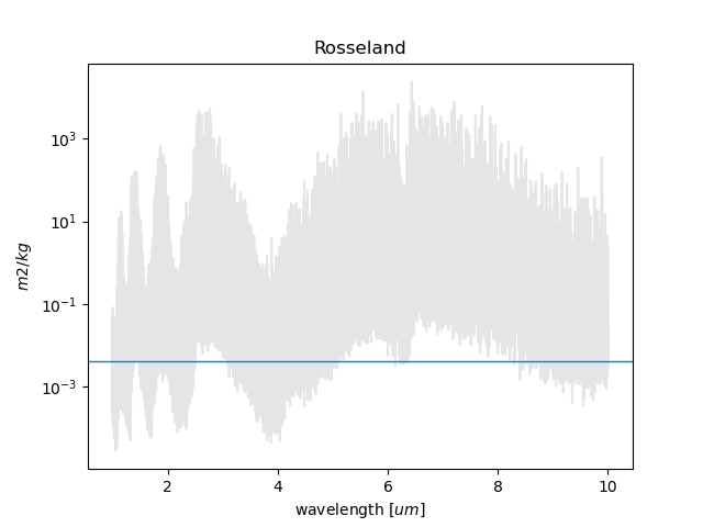
If instead multiple opacities have been calculated, then then the script should be:
P = [1, 10 ] *u.bar
T = [500.0, 1000.0, 2000.0] *u.K
wl = (1 * u.um, 10 * u.um)

fig0, ax0 = ross.estimate_plot(P_input = P, T_input=T, band=wl, mode='closest')
fig1, ax1 = plan.estimate_plot(P_input = P, T_input=T, band=wl, mode='closest')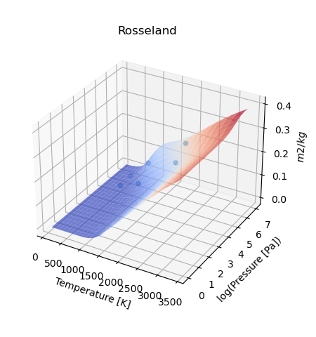
Notwithstanding, to force the production of a map_plot() with a single value,
the following should be used force_map=True
Include Rayleigh scattering
Initialising Rayleigh data
RAPOC can estimate the Rayleigh scattering absorption for a list of atoms, using the tables and equations in Chapter 10 of David R. Lide, ed., CRC Handbook of Chemistry and Physics, Internet Version 2005, hbcponline, CRC Press, Boca Raton, FL, 2005.
To compute the Rayleigh scattering mean opacities, the first step is to produce the Rayleigh data set.
This can be done initialising the Rayleigh class. This class is similar to a
FileLoader class: it can be injected into a Model as input data,
and therefore used as any other input data to estimate the mean opacities.
To initialise the Rayleigh it is needed the atom and the wavenumber grid to use to sample the Rayleigh scattering.
In the following example we estimate the scattering data for hydrogen in a simple wavenumber grid: 100000, 10000, 1000 cm-1
from rapoc import Rayleigh
rayleigh = Rayleigh('H', wavenumber_grid=[100000, 10000, 1000])
Another way to initialise the Rayleigh is to use an already initialised Model.
This can be useful is the Rayleigh scattering is to be used along with other absorptions. Let’s assume that a
Planck class has been initialised already.
That model can be used to produce a Rayleigh scattering dataset sampled at the same wavenumbers grid.
plan = Planck(input_data=input_file)
rayleigh = Rayleigh('H', model=plan)
Once the wavenumber grid is produced, either using the wavenumber_grid or the model keyword, the class produces the
opacities data using the compute_opacities().
Estimating Rayleigh mean opacities
The initialised Rayleigh can be now used as input data for Rosseland and
Planck
ross = Rosseland(input_data=rayleigh)
plan = Planck(input_data=rayleigh)
Because the Rayleigh scattering doesn’t depend on temperature and pressure, is not sampled in a temperatures and pressures grid as the molecular opacities. Therefore, to estimate its mean opacities the pressure must not be indicated. The temperature, on the contrary, must be indicated because of the Rosseland and Planck equation involving a black body. For the same reason, the estimation mode is forced to closest, so should not be indicated by the user. Here is an example
T = 1000.0 *u.K
wl = (1 * u.um, 10 * u.um)

r_estimate = ross.estimate(T_input=T, band=wl)

6.725572872420127e-08 m2 / kg
p_estimate = plan.estimate(T_input=T, band=wl) 6.518714389415313e-09 m2 / kg
Because, again, the Rayleigh scattering doesn’t depend on temperature and pressure, the map()
is disabled for this kind of data